We have been discussing the variability in feed ingredient costs and how we often disregard it in the traditional ways we estimate our cost of production or projections of cash flow. It is common to use the current or average price over some previous period of time to calculate current cost of production or to forecast the future value of feed ingredient costs, as an example.
The problem with this approach is we live in a time of tremendous price variability and representing the likely journey of price levels over time with a single value can lead to poor decision-making. Many decisions we take in production require multi-period analysis (such as asset investment, expansion, forward pricing) and glossing over the range of possible price outcomes is like taking flight with only enough fuel to make the journey in average conditions. A stiff head wind, a hold for a thunderstorm over the airport or departure delays due to traffic congestion can lead to a very vulnerable situation.

Fortunately, there are some basic tools to assess variability in the planning process and we can go through an example which will demonstrate the value of doing just that.
If we knew the pattern within which prices were likely to move over time, we could enhance our analysis by running several versions of our budgets or cash flow forecasts using that pattern and trace out the full range of outcomes which are possible. This is part of a set of techniques called sensitivity analysis. In its most basic form, sensitivity analysis involves running three versions of your forecasts, an expected version, a “worst-case” and a “best-case” version. This is a big improvement from single value budgeting as it provides a means to evaluate what might happen if things go differently than expected. For instance, a plausible “worst-case” run of your budgets may suggest that you need to negotiate an additional 25% cushion in your line of credit request up front. Lenders really appreciate borrowers who think ahead and most will not mind approving extra capacity at the beginning of your project if you can show your request is the result of careful and prudent budgeting which takes into account the range of possible outcomes, rather than only the most likely. It is much easier to get approvals for this cushion up front rather than to request additional capital when things are turning against you later.
Beyond the three-part approach to sensitivity analysis is a more sophisticated version involving estimating the pattern of future prices from previous price movements and your knowledge of the future. Once you have characterized these expected patterns, called “distributions” of expected prices, you can use the computer to generate hundreds or even thousands of runs of your budgets taking random samples from the pattern of price movements you believe are likely to occur and testing the result. This is referred to as a simulation analysis. The results of this large number of sample runs can be easily summarized as its own distribution of likely outcomes and with this distribution, a probability of achieving each level of outcome can be assigned.
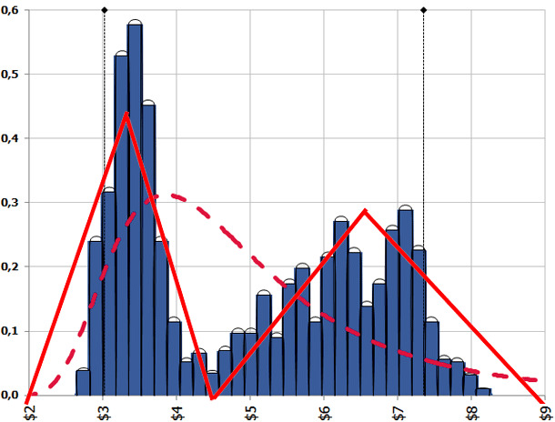
Take a look at Figure 1. It shows the distribution of actual U.S. corn prices per bushel since January of 2007. I chose 2007 as a beginning point since the effect of ethanol demand for corn became a permanent factor in U.S. corn prices in late 2006. Using corn prices before 2006 would probably not provide sound information for forecasting the future. The blue regions of Figure 1., depict the historical frequency pattern for each price. Note that there are three different peaks (called modes) in this distribution. The price with the highest frequency of occurrence is around $3.50 per bushel (major mode). The other two high frequency occurrences are around $6.20 and $7.00/bu (minor modes). I have illustrated with the red lines, two plausible ways to characterize the overall frequency of prices to use in our simulation runs. You can preserve the multi-modal frequency or smooth over it to produce a skewed, single mode distribution.
Figure 1. US Corn Prices $/BU 2007- 2013 Partial
Using the smoothed version of the corn distribution and a similar one for soybean meal prices, I can substitute those distributions into a set of standard finishing diets in place of the single average price estimate for corn and bean meal and produce a distribution of expected feed costs. For simplicity in this demonstration, I fix the minor feed ingredient prices and ratio a few more important ones to the corn and bean meal prices in their usual relationship. This is a shortcut which you would not necessarily want to do for an actual forecast but it makes our bigger point without a lot of complexities to handle in a short article. The corn price distribution has a mean price of $4.83/bu and a standard deviation of $1.58. The soybean meal price distribution has a mean price of $348.70/ US ton and a standard deviation of $81.89. Just from that we know that if we use only the mean value to forecast a particular outcome, we would expect to be off, on average, an amount equal to the standard deviation of each price. We live in a time of high price variability.
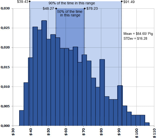
Figure 2. illustrates the result of our finishing feed cost estimation on pig basis. This is the result of 1,000 estimations of our feed cost budgets using random selections of price pairs from the (correlated) corn and soybean meal price distributions described above. One of the advantages is that you can assign probability estimates to ranges of possible outcomes. In this case, we show the range of prices which we expect our price to fall within both 50 and 90 percent of the time. This provides a means to demonstrate to lenders the stability of our expected costs (and therefore profits) and the range of potential working capital requirements we expect over the next planning period. It also clearly shows what we have already discovered, if there is a deviation from the more “normal” range of prices, it is more likely to be a deviation to the high cost side. This is illustrated by the right hand tail being longer and flatter.
Figure 2. Distribution of Estimated Finishing Feed Cost/Pig 2014